Support Vector Machine
So far in both regression and classification problems, we have used probabilistic predictors. Here,
we learn a non-probabilistic method, which is known as Support Vector Machines (SVMs).
This margin-based approach often leads to strong generalization, especially in high dimensional spaces with limited
samples. By employing the kernel trick (e.g., RBF kernel), SVMs can implicitly map inputs
into higher dimensional feature spaces, enabling the classification of nonlinearly separable data without explicitly
computing those transformations. Despite the rise of deep learning, SVMs remain valuable for small- to medium-sized
datasets, offering robustness and interpretability through a sparse set of support vectors.
In binary classification \(h(x) = \text{sign }(f(x))\), the decision boundary (hyperplane) is given by:
\[
f(x) = w^\top x + w_0 \tag{1}
\]
To obtain robust solution, we would like to maximize the margin between data points and the decision boundary.
To express the distance of the closest point to the decision boundary,
we introduce the orthogonal projection of any point \(x\) onto the boundary \(f(x)\):
\[
x = \text{proj}_{f(x)}x + r \frac{w}{\| w \|} \tag{2}
\]
where \(r\) is the distance from \(x\) to the decision boundary whose normal vector is \(w\).
Substitute Expression (2) for the decision boundary (1):
\[
\begin{align*}
f(x) &= w^\top \left(\text{proj}_{f(x)}x + r \frac{w}{\| w \|} + w_0 \right) \\\\
&= w^\top \text{proj}_{f(x)}x + w_0 + r \| w \|.
\end{align*}
\]
Since \(f(\text{proj}_{f(x)}x ) = 0\),
\[
r = \frac{f(x)}{\| w \|}
\]
and each point must be on the correct side of the decision boundary:
\[
f(x_n)\tilde{y}_n > 0.
\]
Therefore, our objective is represented by:
\[
\max_{w, w_0} \frac{1}{\| w \|} \min_{n = 1}^N \left[\tilde{y}_n \left(w^\top x_n + w_0 \right)\right].
\]
Moreover, define a scale factor \(k\) subject to \(\tilde{y}_n f_n =1\), but the scaling does not change the
distance of points to the decision boundary (it will be canceled out by \(\frac{1}{\| w \|}\) ).
Note that \(\max \frac{1}{\| w \|}\) is the same as \(\min \| w \|^2\). Thus our objective becomes:
\[
\min_{w, w_0} \frac{1}{2}\| w \|^2
\]
subjec to
\[
\tilde{y}_n (w^\top x_n + w_0) \geq 1, \quad n = 1 : N.
\]
(Factor of \(\frac{1}{2}\) is for just convenience.)
This constrained optimization problem, known as the primal problem, is difficult to solve directly. However,
since this is the convex optimization problem, there exists its dual problem
using Lagrange multipliers, which often has computational advantages and enables the kernel trick.
Let \(\alpha \in \mathbb{R}^N\) be the dual variables corresponding to Lagrange multipliers:
\[
\mathcal{L}(w, w_0, \alpha) = \frac{1}{2}w^\top w - \sum_{n =1}^N \alpha_n (\tilde{y}_n (w^\top x_n + w_0) -1) \tag{3}
\]
To optimize this, we need a stationary point that satisfies:
\[
(\hat{w}, \hat{w_0}, \hat{\alpha}) = \min_{w, w_0} \max_{\alpha} \mathcal{L}(w, w_0, \alpha).
\]
Taking derivatives wrt \(w\) and \(w_0\) and seting to zero:
\[
\begin{align*}
\nabla_w \mathcal{L}(w, w_0, \alpha) &= w - \sum_{n =1}^N \alpha_n \tilde{y}_n x_n \\\\
\frac{\partial \mathcal{L}(w, w_0, \alpha)}{\partial w_0} &= - \sum_{n =1}^N \alpha_n \tilde{y}_n.
\end{align*}
\]
Then we have:
\[
\begin{align*}
\hat{w} &= \sum_{n =1}^N \hat{\alpha_n} \tilde{y}_n x_n \\\\
0 &= \sum_{n =1}^N \hat{\alpha_n} \tilde{y}_n.
\end{align*}
\]
Substitute these for the Lagrangian (3), we obtain
\[
\begin{align*}
\mathcal{L}(\hat{w}, \hat{w_0}, \alpha) &= \frac{1}{2}\hat{w}^\top \hat{w} - \sum_{n =1}^N \alpha_n \tilde{y}_n \hat{w}^\top x_n
- \sum_{n =1}^N \alpha_n \tilde{y}_n w_0 + \sum_{n =1}^N \alpha_n \\\\
&= \frac{1}{2}\hat{w}^\top \hat{w} - \hat{w}^\top \hat{w} - 0 + \sum_{n =1}^N \alpha_n \\\\
&= - \frac{1}{2} \sum_{i =1}^N \sum_{j = 1}^N \alpha_i \alpha_j \tilde{y}_i \tilde{y}_j x_i^\top x_j
+ \sum_{n =1}^N \alpha_n.
\end{align*}
\]
Therefore the dual problem is:
\[
\max_{\alpha} \mathcal{L}(\hat{w}, \hat{w_0}, \alpha)
\]
subject to
\[
\sum_{n =1}^N \alpha_n \tilde{y}_n = 0 \text{ and } \alpha_n \geq 0, \quad n = 1 : N.
\]
Also, the solution must satisfy the KKT conditions:
\[
\begin{align*}
\alpha_n &\geq 0 \text{ (Dual feasibility) }\\\\
\tilde{y}_n f(x_n) -1 &\geq 0 \text{ (Primal feasibility) }\\\\
\alpha_n (\tilde{y}_n f(x_n) -1 ) &= 0 \text{ (Complementary slackness) }
\end{align*}
\]
Thus, for each data point, either
\[
\alpha_n = 0 \, \text{ or } \, \tilde{y}_n (\hat{w}^\top x_n + \hat{w}_0) = 1
\]
must hold. The points meet the second condition are called support vectors.
Let the set of support vectors be \(\mathcal{S}\). To perform prediction, we use:
\[
\begin{align*}
f(x ; \hat{w}, \hat{w}_0) &= \hat{w}^\top x + \hat{w}_0 \\\\
&= \sum_{n \in \mathcal{S}} \alpha_n \tilde{y}_n x_n^\top x + \hat{w}_0.
\end{align*}
\]
By the kernel trick,
\[
f(x) = \sum_{n \in \mathcal{S}} \alpha_n \tilde{y}_n \mathcal{K}(x_n, x) + \hat{w}_0
\]
Also,
\[
\begin{align*}
\hat{w}_0 &= \frac{1}{|\mathcal{S}|} \sum_{n \in \mathcal{S}} \left(\tilde{y}_n - \hat{w}^\top x_n \right) \\\\
&= \frac{1}{|\mathcal{S}|} \sum_{n \in \mathcal{S}} \left(\tilde{y}_n - \sum_{m \in \mathcal{S}} \alpha_m \tilde{y}_m x_m^\top x_n \right).
\end{align*}
\]
By the kernel trick,
\[
\frac{1}{|\mathcal{S}|} \sum_{n \in \mathcal{S}} \left(\tilde{y}_n - \sum_{m \in \mathcal{S}} \alpha_m \tilde{y}_m \mathcal{K}(x_m, x_n) \right).
\]
Soft Margin Constraints
Consider the case where the data is NOT linearly separable. In this case there is not feasible solution in which
\(\forall n, \, \tilde{y}_n f_n \geq 1\). By introducing slack variables \(\xi_n \geq 0\), we relax
the constraints \(\tilde{y}_n f_n \geq 0\) with soft margin constraints:
\[
\tilde{y}_n f_n \geq 1 - \xi_n
\]
Thus our objective becomes:
\[
\min_{w, w_0, \xi} \frac{1}{2} \| w \|^2 + C \sum_{n =1}^N \xi_n
\]
subject to
\[
\xi_n \geq 0, \quad \tilde{y}_n (x_n^\top w + w_0) \geq 1 - \xi_n
\]
where \(C \geq 0\) is a hyper parameter that controls how many data points are allowed to violate the margin.
The Lagrangian becomes:
\[
\begin{align*}
&\mathcal{L}(w, w_0, \alpha, \xi, \mu) \\\\
&= \frac{1}{2} w^\top w + C \sum_{n =1}^N \xi_n
- \sum_{n = 1}^N \alpha_n (\tilde{y}_n(w^\top x_n + w_0) -1 + \xi_n)
- \sum_{n = 1}^N \mu_n \xi_n
\end{align*}
\]
where \(\alpha_n \geq 0, \text{ and } \mu_n \geq 0\) are lagrange multipliers.
By optimizing out \(w, \, w_0, \text{ and } \xi\), we obtain:
\[
\mathcal{L}(\alpha) = \sum_{i = 1}^N \alpha_i -\frac{1}{2}\sum_{i =1}^N \sum_{j = 1}^N \alpha_i \alpha_j \tilde{y}_i \tilde{y}_j x_i^\top x_j.
\]
This dual form is equivalent to the hard margin version, but constraints are different. By the KKT conditions:
\[
0 \leq \alpha_n \leq C
\]
\[
\sum_{n=1}^N \alpha_n \tilde{y}_n = 0
\]
These constraints imply:
- If \(\alpha_n = 0\), the point is ignored.
- If \(0 < \alpha_n < C\), the point is on the margin. (\(\xi_n = 0\))
- If \(\alpha_n = C\), the point is inside the margin. In this case,
- If \(\xi_n \leq 1\), the point is correctly classified.
- If \(\xi_n > 1\), the point is misclassified.
SVM Demo
This interactive demo visualizes the SVM algorithm in action. You can observe how the algorithm finds the optimal
decision boundary that maximizes the margin between two classes while respecting the soft margin constraints.
Understanding the Visualization
The visualization displays several key components of the SVM:
- Training Data Points: Solid circles represent training samples with labels \(\tilde{y} \in \{-1, +1\}\)
- Test Data Points: Semi-transparent squares show test samples for evaluating generalization
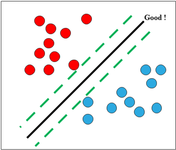
- Decision Boundary: The dark line (linear kernel) or contour (RBF kernel) where \(f(x) = w^\top x + w_0 = 0\)
- Margin Boundaries: Dashed lines showing where \(\tilde{y}_n f(x_n) = 1\)
- Support Vectors: Points with golden borders that satisfy \(\alpha_n > 0\) and define the decision boundary
- Slack Variables: Dotted circles around support vectors visualize \(\xi_n\) for points violating the margin
Interactive Controls
Experiment with different parameters to understand their effects:
- Kernel Type:
- Linear: Uses \(\mathcal{K}(x_i, x_j) = x_i^\top x_j\) for linearly separable data
- RBF (Gaussian): Uses \(\mathcal{K}(x_i, x_j) = \exp(-\gamma \|x_i - x_j\|^2)\) for non-linear boundaries
- Regularization Parameter C: Controls the trade-off between maximizing the margin and minimizing classification errors.
As shown in the soft margin formulation: \(\min_{w, w_0, \xi} \frac{1}{2} \| w \|^2 + C \sum_{n =1}^N \xi_n\)
- Low C: Prioritizes wider margins, allows more margin violations
- High C: Prioritizes correct classification, may lead to overfitting
- RBF Gamma (γ): Controls the influence radius of support vectors in RBF kernel
- Low γ: Smooth decision boundaries, each point influences a wider region
- High γ: Complex boundaries, localized influence around each support vector
- Learning Rate & Iterations: SGD optimization parameters for training convergence
Training Process
The demo uses Stochastic Gradient Descent (SGD) to optimize the SVM objective. For the RBF kernel, it employs
Random Fourier Features to approximate the kernel function, making the non-linear SVM computationally efficient.
Click "Train SVM" to watch the algorithm iteratively:
- Update weights to minimize the hinge loss: \(\max(0, 1 - \tilde{y}_n f(x_n))\)
- Apply regularization to control model complexity
- Identify support vectors that satisfy the KKT conditions
- Converge to the optimal decision boundary
Observing KKT Conditions
After training, the demo verifies the Karush-Kuhn-Tucker (KKT) conditions for each point:
- For non-support vectors (\(\alpha_n = 0\)): Must have \(\tilde{y}_n f(x_n) \geq 1\)
- For support vectors on the margin (\(0 < \alpha_n < C\)): Must have \(\tilde{y}_n f(x_n) = 1\)
- For support vectors inside/beyond margin (\(\alpha_n = C\)): May have \(\tilde{y}_n f(x_n) < 1\)
The percentage of points satisfying these conditions indicates how well the optimization has converged.
Experiment Suggestions
Try these experiments to deepen your understanding:
- Generate linearly separable data and compare linear vs RBF kernels
- Create circular data patterns to see where linear kernels fail
- Adjust C to observe the trade-off between margin width and training accuracy
- For RBF kernel, vary γ to see how decision boundaries become more complex
- Watch how the number of support vectors changes with different parameters