The graph Laplacian is a matrix representation that captures the structure of a graph
and plays a central role in spectral graph theory. Building on your knowledge of
graph theory and eigenvalues,
we'll explore how the Laplacian encodes connectivity patterns and enables powerful analytical techniques.
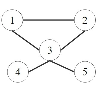
If \(G\) is a graph with vertex set \(\{1, 2, \ldots, n-1, n\}\). Let \(D(G)\) be the \(n \times n\) diagonal
matrix of vertex degrees of \(G\). The Laplacian matrix is defined as
\[
L(G) = D(G) - A(G)
\]
where \(A(G)\) is the adjacency matrix of \(G\).
Moreover, the spectral decomposition of the Laplacian matrix \(\boldsymbol{L}\) reveals deeper structure and provides a
spectral interpretation of smoothness on graphs.
Since \(\boldsymbol{L}\) is symmetric and positive semi-definite, it admits an orthonormal eigendecomposition:
\[
\boldsymbol{L} = \boldsymbol{V}\,\boldsymbol{\Lambda}\,\boldsymbol{V}^\top,
\quad
\boldsymbol{\Lambda} = \mathrm{diag}(\lambda_1, \lambda_2, \dots, \lambda_N),
\]
with ordered eigenvalues
\[
0 = \lambda_1 \le \lambda_2 \le \cdots \le \lambda_N,
\]
and orthonormal eigenvectors \(\boldsymbol{v}_1, \dots, \boldsymbol{v}_N\) forming a complete basis for functions defined on the graph.
Several important spectral properties follow:
The multiplicity of the zero eigenvalue equals the number of connected components in the graph.
For a connected graph, \(\lambda_1 = 0\) is simple, and its eigenvector is proportional to the constant vector \(\boldsymbol{1}\).
The second smallest eigenvalue, \(\lambda_2\), known as the algebraic connectivity (or Fiedler value),
quantifies the graph's overall connectivity: larger \(\lambda_2\) implies stronger connectivity and fewer natural partitions.
For any unit-norm eigenvector \(\boldsymbol{v}_k\),
\[
\boldsymbol{v}_k^\top \boldsymbol{L}\, \boldsymbol{v}_k = \lambda_k,
\]
meaning that eigenvectors with larger eigenvalues correspond to functions of higher “energy” (less smoothness) on the graph.
If an arbitrary function \(\boldsymbol{f}\) is expanded in this eigenbasis as
\[
\boldsymbol{f} = \sum_{k=1}^N \alpha_k \boldsymbol{v}_k,
\]
its Dirichlet energy decomposes as
\[
\boldsymbol{f}^\top \boldsymbol{L}\, \boldsymbol{f} = \sum_{k=1}^N \alpha_k^2 \lambda_k.
\]
Hence, components along higher-\(\lambda\) eigenvectors contribute more to the overall roughness of \(\boldsymbol{f}\).
Spectral Properties and the Fiedler Vector
The eigenvalues of the graph Laplacian provide deep insights into graph structure. For the unnormalized Laplacian \(\mathbf{L}\),
the eigenvalues satisfy \(0 = \lambda_0 \leq \lambda_1 \leq \cdots \leq \lambda_{n-1}\).
The Fiedler Vector and Algebraic Connectivity
The second smallest eigenvalue \(\lambda_1\) is called the algebraic connectivity or Fiedler value.
Its corresponding eigenvector \(v_1\) (the Fiedler vector) has remarkable properties:
\(\lambda_1 > 0\) if and only if the graph is connected
The Fiedler vector provides a natural 1D embedding that tends to separate loosely connected parts
The Spectral Gap and Cheeger's Inequality
The spectral gap \(\lambda_1\) relates to how well-connected the graph is. This is formalized by Cheeger's inequality,
which bounds the relationship between the spectral gap and the graph's expansion properties:
Cheeger's Inequality
For a connected graph, let \(h(G)\) be the Cheeger constant (isoperimetric number):
\[
h(G) = \min_{S \subset V, 0 < |S| \leq n/2} \frac{|\partial S|}{\min(|S|, |V \setminus S|)}
\]
where \(|\partial S|\) is the number of edges between \(S\) and its complement. Then:
\[
\frac{h(G)^2}{2d_{max}} \leq \lambda_1 \leq 2h(G)
\]
This shows that graphs with large spectral gaps have good expansion properties—there are no "bottlenecks" separating the graph into weakly connected parts.
Graph Signal Processing Perspective
The eigenvectors of the Laplacian form a Fourier basis for signals on the graph. For a signal \(f: V \to \mathbb{R}\)
defined on vertices:
Graph Fourier Transform
If \(\mathbf{U} = [u_0, u_1, \ldots, u_{n-1}]\) contains the eigenvectors of \(\mathbf{L}\), the Graph Fourier Transform is:
\[
\hat{f} = \mathbf{U}^T f
\]
and the inverse transform:
\[
f = \mathbf{U} \hat{f}
\]
The eigenvalues \(\lambda_i\) represent "frequencies":
Small \(\lambda_i\) ↔ low frequency (smooth over graph)
Large \(\lambda_i\) ↔ high frequency (oscillatory over graph)
This perspective is crucial for Graph Neural Networks, where spectral methods like ChebNet use polynomial approximations
of spectral filters:
\[
g_\theta(L) = \sum_{k=0}^K \theta_k T_k(\tilde{L})
\]
where \(T_k\) are Chebyshev polynomials and \(\tilde{L} = \frac{2}{\lambda_{max}}L - I\) is the scaled Laplacian.
Connection to Random Walks and Diffusion
The normalized Laplacian connects to random walks and diffusion processes on graphs:
Heat Diffusion on Graphs
The heat equation on a graph is:
\[
\frac{\partial u}{\partial t} = -\mathbf{L} u
\]
with solution:
\[
u(t) = e^{-t\mathbf{L}} u(0) = \sum_{i=0}^{n-1} e^{-t\lambda_i} \langle u(0), v_i \rangle v_i
\]
This shows how initial heat distribution \(u(0)\) diffuses over the graph, with convergence rate determined by \(\lambda_1\).
Computational Considerations for Large Graphs
For graphs with millions of nodes (common in 2025 applications), exact eigendecomposition is infeasible.
Modern approaches include:
Lanczos Algorithm: Iteratively finds top-k eigenvectors in \(O(kn)\) per iteration
Power Iteration: Simple method for dominant eigenvector, basis for PageRank
Chebyshev Polynomial Approximation: Avoids eigendecomposition entirely:
\[
T_k(x) = 2xT_{k-1}(x) - T_{k-2}(x)
\]
Used in Graph Convolutional Networks (GCNs) for scalable spectral filtering
Random Projection Methods: Johnson-Lindenstrauss based approaches for approximate embeddings
Modern Applications Beyond Clustering
Graph Laplacians are fundamental to many 2025 AI applications:
Graph Neural Networks: GCN uses \(\tilde{L} = I - D^{-1/2}AD^{-1/2}\) for message passing
Recommender Systems: Netflix/YouTube use spectral methods on user-item graphs
Protein Structure: AlphaFold uses graph representations with Laplacian-based features
Social Network Analysis: Community detection via spectral clustering at Facebook/LinkedIn scale
Computer Vision: Superpixel segmentation and image denoising via graph cuts