Gaussian Function
A Gaussian function is defined as:
\[
f(x) = e^{-x^2}
\]
and often is parametrized as
\[
f(x) = a e^{-\frac{(x-b)^2}{2c^2}} \tag{1}
\]
where \(a, b , c \in \mathbb{R}, \text{ and } c \neq 0\).
The family of Gaussian functions does not have elementary antiderivatives. To represent the integral of Gaussian functions,
we use the special function known as the error function:
\[
\text{erf }(z) = \frac{2}{\sqrt{\pi}} \int_{0}^z e^{-t^2}dt. \qquad \text{erf}: \mathbb{C} \to \mathbb{C}
\]
Then,
\[
\int e^{-x^2} dx = \frac{\sqrt{\pi}}{2}\text{erf }(x) + C.
\]
On the other hand, their improper integrals over \(\mathbb{R}\) can be evaluated exactly using Gaussian integral:
Theorem 1: Gaussian Integral
\[
\int_{-\infty} ^\infty e^{-x^2} dx = \sqrt{\pi}.
\]
Note: The generalized Gaussian integral is given by
\[
\int_{-\infty} ^\infty e^{-ax^2} dx = \sqrt{\frac{\pi}{a}} \qquad a > 0 \tag{2}
\]
Proof:
Let \(I = \int_{-\infty} ^\infty e^{-x^2} dx\). Then
\[
\begin{align*}
I^2 &= \int_{-\infty} ^\infty \int_{-\infty} ^\infty e^{-u^2} e^{-v^2} du dv \\\\
&= \int_{-\infty} ^\infty \int_{-\infty} ^\infty e^{-(u+v)^2} dudv.
\end{align*}
\]
Using the polar coordinates, let \(u = r\cos \theta\), and \(v = r\sin \theta\) and then
\(u^2 + v^2 = r^2\) and \(dudv = r dr d\theta\).
Thus,
\[
\begin{align*}
I^2 &= \int_{0} ^{2\pi} \int_{0} ^\infty e^{-r^2} r dr d\theta \\\\
&= \int_{0} ^{2\pi} 1d\theta \int_{0} ^\infty e^{-r^2} r dr. \\\\\
\end{align*}
\]
Here, let \(w = -r^2\) and \(dw = -2rdr\). Then
\[
\begin{align*}
I^2 &= (2\pi) (-\frac{1}{2}\int_{0} ^{-\infty} e^{w} dw) \\\\\
&= (2\pi) (\frac{1}{2}\int_{-\infty} ^0 e^{w} dw)\\\\\
&= (2\pi)(\frac{1}{2}\cdot 1)
\end{align*}
\]
Therefore,
\[
I = \sqrt{\pi}.
\]
This is the case where \(a =1\) in the generalized Gaussian integral. We extend this result to the
generalized case with a scaling factor \(a>0\).
Let \(u = sqrt{a}x\) and then \(x = \frac{u}{\sqrt{a}} \) and \(dx = \frac{1}{\sqrt{a}}du\).
Substituting these into the integral (2)
\[
\begin{align*}
& \int_{-\infty} ^\infty e^{-a(\frac{u}{\sqrt{a}})^2} \frac{1}{\sqrt{a}}du \\\\
&= \frac{1}{\sqrt{a}} \int_{-\infty} ^\infty e^{-u^2}du \\\\
&= \frac{1}{\sqrt{a}} (\sqrt{\pi}) \\\\
&= \sqrt{\frac{\pi}{a}}
\end{align*}
\]
Here, we use the parametrized Gaussian function (1).
Let \(u = \frac{x-b}{c}\), which implies \(x = cu + b \) and \(dx = cdu\). Then
\[
\begin{align*}
\int_{-\infty} ^\infty a e^{-\frac{(x-b)^2}{2c^2}} dx
&= \int_{-\infty} ^\infty a e^{-\frac{(cu)^2}{2c^2}}cdu \\\\
&= ac \int_{-\infty} ^\infty e^{-\frac{u^2}{2}}du
\end{align*}
\]
Using the Gaussian integral (3),
\[
\begin{align*}
\int_{-\infty} ^\infty a e^{-\frac{(x-b)^2}{2c^2}} dx
&= ac \int_{-\infty} ^\infty e^{-\frac{u^2}{2}}du \\\\
&= ac\sqrt{2\pi}. \tag{3}
\end{align*}
\]
Normal(Gaussian) Distribution
A random variable \(X\) has a normal(Gaussian) distribution with parameters \(\mu \) and
\(\sigma^2\) if its p.d.f. is given by
\[
f(x) = \frac{1}{\sigma \sqrt{2\pi}}e^{\frac{-(x - \mu)^2}{2\sigma^2}} \qquad x \in \mathbb{R}
\]
where \(\mu \in \mathbb{R}\) and \(\sigma > 0\) and it is denoted as \(X \sim N(\mu, \sigma^2)\).
Note that the c.d.f. of the normal distribution does not have closed form:
\[
F(x) = \int_{-\infty} ^\infty \frac{1}{\sigma \sqrt{2\pi}}e^{\frac{-(x - \mu)^2}{2\sigma^2}}
\]
but comparing with the expression (3), this is the gaussian integral with \(a = \frac{1}{c\sqrt{2\pi}}, \,
b = \mu, \text{ and } c = \sigma\) to make its value \(1\).
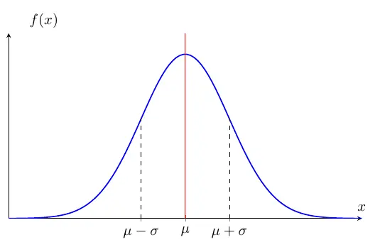
The above figure shows the normal p.d.f. curve. \(\mu\) is the center, and \(\sigma\) is the distance from
the center to the inflection point of the curve. The one reason the normal distribution is widely used in statistics
and machine learning as well, the parameters capture its mean and variance, which are essential properties of the distribution.
\[
\mathbb{E }[X] = \mu \qquad \text{Var }(X) = \sigma^2.
\]
So, in the normal distribution, measures of central tendency(mean, median, and mode) are the same.
The simplest and useful normal distribution is the one with zero mean and unit variance. We call it
the standard normal distribution denoted by
\[
Z \sim N(0, 1).
\]
Any normally distributed random variable can be "transformed" to a standard normal random variable. If
\(X \sim N(\mu, \sigma^2)\), then
\[
Z = \frac{X- \mu}{\sigma}\sim N(0, 1).
\]
This process is called standardization. This is just a special case of the linear transformation:
\[
Y = aX + b \sim N(a\mu+b, a^2\sigma^2)
\]
Here, \(a = \frac{1}{\sigma} \) and \(b = \frac{-\mu}{\sigma}\) and then you
get \(\mathbb{E}[\frac{1}{\sigma}x -\frac{\mu}{\sigma}] = 0 \) and \(\text{Var }(\frac{1}{\sigma}x -\frac{\mu}{\sigma}) =1\).
The p.d.f. of \(Z\) is denoted by
\[
\phi (z) = f(x) = \frac{1}{\sqrt{2\pi}}e^{\frac{-z^2}{2}} \qquad z \in \mathbb{R}
\]
and c.d.f. of \(Z\) is denoted by
\[
\Phi (z) = P(Z \leq z) = \int_{-\infty} ^z \phi (u)du.
\]
Central Limit Theorem
Now, we consider a set of random variables \(\{X_1, X_2, \cdots, X_n\}\). In random sampling, we assume that each
\(X_i\) has the same distribution and is independent of each other. We call it independent and identically distributed(i.i.d.).
In this case, a single sample mean \(\bar{X} = \frac{1}{n}\sum_{i=1} ^n X_i\) is not exactly equivalent to the population mean \(\mu\)
because there are many different sampling possibilities. However, the "average" of sample means is equal to \(\mu\):
\[
\begin{align*}
\mathbb{E}[\bar{X}] &= \mathbb{E}[\frac{1}{n}(X_1 + X_2 + \cdots +X_n)] \\\\
&= \frac{1}{n}[\mathbb{E}[X_1] + \mathbb{E}[X_2] + \cdots + \mathbb{E}[X_n]] \\\\
&= \frac{n\mu}{n} \\\\
&= \mu
\end{align*}
\]
Thus, the sample mean is an unbiased estimator of the population mean \(\mu\). On the other hand,
the sample variance \(s^2\) is a biased estimator of the population variance \(\sigma^2\):
\[
\begin{align*}
\text{Var }(\bar{X}) &= \text{Var }[\frac{1}{n}(X_1 + X_2 + \cdots +X_n)] \\\\
&= \frac{1}{n^2}[\text{Var }(X_1) + \text{Var }(X_2) + \cdots + \text{Var }(X_n)] \\\\
&= \frac{n \sigma^2}{n^2} \\\\
&= \frac{\sigma^2}{n}
\end{align*}
\]
To make the estimator unbiased, we adjust the denominator:
\[
s^2 = \frac{1}{n-1} \sum_{i=1}^n (X_i - \bar{X})^2.
\]
At this point, you might wonder how we can make inferences about the unknown distribution of random variables in practice.
The Central Limit Theorem (CLT) provides a result: regardless of the underlying distribution of a population,
the distribution of the sample mean approaches a normal distribution as the sample size \(n\) becomes large enough. This remarkable
property is one of the reasons the normal distribution is widely used in statistics and forms the foundation of many statistical methods
and theories.
Theorem 1: Central Limit Thorem
Let \(X_1, X_2, \cdots, X_n\) be i.i.d. random variables with mean \(\mu\) and variance \(\sigma^2\). Then the distribution of
\[
Z = \frac{\bar{X} - \mu}{\frac{\sigma}{\sqrt{n}}}
\]
converges to the standard normal distribution as the smaple size \(n \to \infty\).
Note: The SD of \(\bar{X}\) is \(\sqrt{\frac{\sigma^2}{n}} = \frac{\sigma}{\sqrt{n}}\).
If the smaple size \(n\) is large enough,
\[
\bar{X} \sim N(\mu, \frac{\sigma^2}{n})
\]
and also,
\[
\sum_{i =1} ^n X_i \sim N(n\mu , n\sigma^2).
\]
Note: For example, highly skewed distributions such as the exponential distribution requires
around \(n \geq 100\) for applying CLT.